Finance

Cohort-based LTV

Cohort-based LTV values a customer by following real groups of customers acquired in the same period and projecting how many will still be paying in each future period, instead of dividing margin by one average churn rate.

In short

Cohort-based LTV is the expected profit from a customer, calculated from how a group of customers acquired in the same period actually stays over time. You add up margin times the share still active in each period, with the observed months taken from data and the later months projected. It avoids the error of applying one average churn rate to customers who leave at very different speeds.

Origin: Peter Fader and Bruce Hardie (probability models of retention and repeat buying); Sunil Gupta, Donald Lehmann and Jennifer Stuart (customer-base valuation), 2004 to 2010
Level: 201 · Tool
Fits: Small and mid-size, Scale-up
Time to apply: One to two days for a first cohort table and a projection, then a quarterly refresh
What you need: a start date for each customer and a dated record of when they stop or stay active · margin per active customer per period, after the variable cost of serving them · at least one cohort old enough to show whether retention flattens, plus a discount rate your finance lead accepts

Cohort-based LTV is a way of valuing a customer from the observed behavior of a group acquired in the same period. You follow the group, count how many are still active at each age, multiply by margin, discount, and project the ages the data has not reached yet. It sits between the quick formula of margin divided by churn and a full forecasting model, and it is the version that unit economics reviews and customer-based valuations rely on. Peter Fader and Bruce Hardie built most of the method; Gupta, Lehmann and Stuart set out the cohort-level valuation logic that it refines.

Why does one average churn rate misstate LTV?

Because the customers in a cohort leave at different speeds, so the churn you measure early is not the churn that applies later. Quick leavers go first. The people who remain are the slow leavers, and the cohort’s retention rate rises even though no individual changes. A single rate then overstates losses in the tail and undervalues the cohort.

Fader and Hardie’s 2010 paper builds the case with a stylized firm. One third of customers keep 90% a year and two thirds keep 50%. Year by year the cohort retains 63.3%, 68.9%, 74.7% and 79.8%. A student applying the textbook formula pools all cohorts into one rate of 69.1% and values the customer base at about $4.95 million. The segment-aware figure is $7.94 million, so the textbook answer is 38% too low.

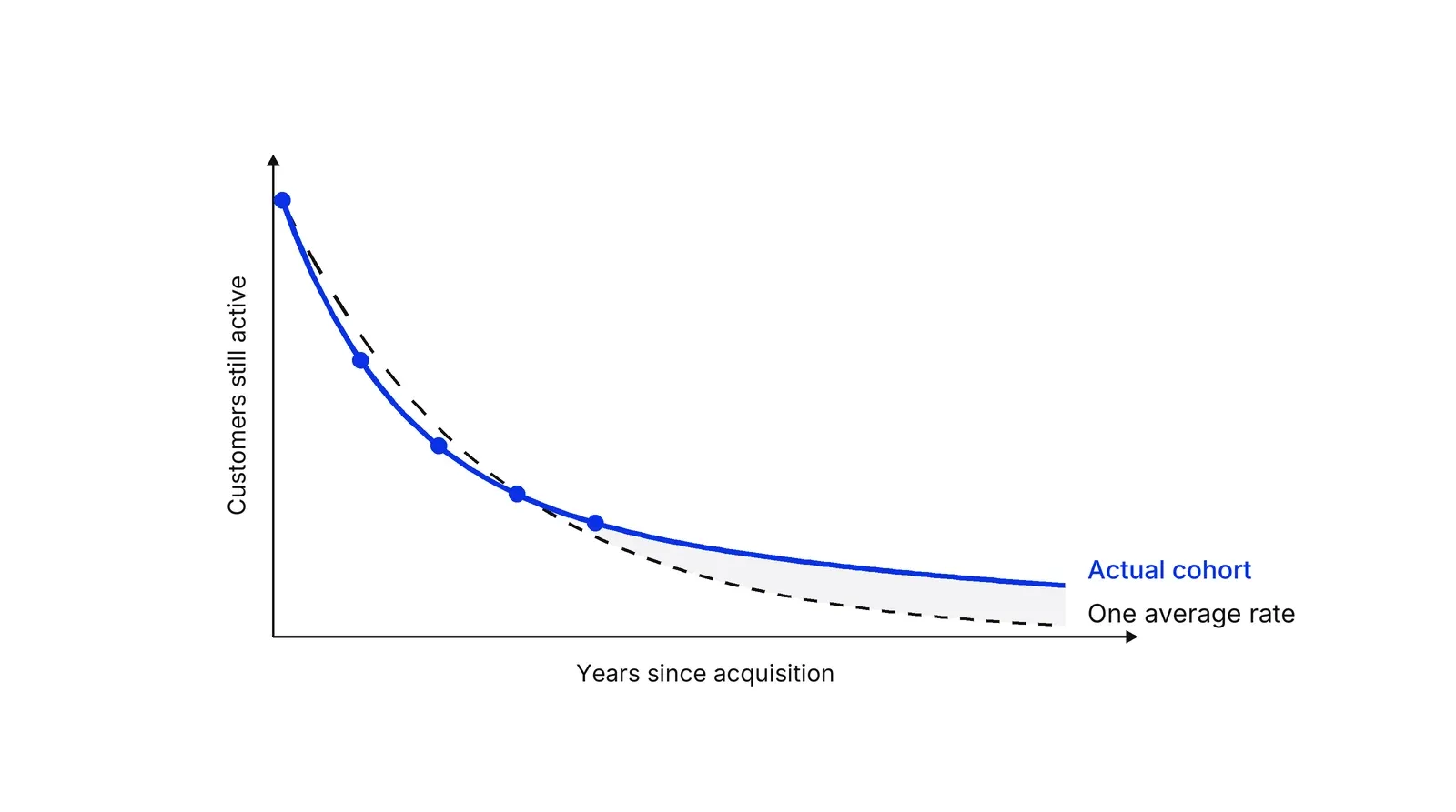
A line chart of customers still active against years since acquisition. A blue line for the actual cohort drops and flattens, with dots on the first five observed years. A dashed black line for one average rate follows it closely for four years, then falls below it, and the gap between the two is shaded grey. — The single rate fits the observed years, then falls away from the cohort in the years nobody has measured yet.

The chart shows why the error hides. Up to the fifth point the dashed line is close, so a check against history passes. The damage sits in the shaded tail, which is where much of the value lives.

Real data behaves the same way. In the shifted beta-geometric paper, a subscription segment keeps 63.1% of customers after year one and 17.3% after year twelve. Holding the year-one rate constant would leave 0.4% at year twelve, which our arithmetic gives from the published table. Fader and Hardie’s source for the idea is Vaupel and Yashin’s 1985 paper on how selection inside a population distorts the aggregate curve.

What does each cohort look like once heterogeneity is counted?

Older cohorts are worth more per customer than the average suggests, because they have already shed their quick leavers. In the same stylized case, a customer from the 2003 cohort still active in 2007 has an expected residual value of $430, and a 2007 customer $226. The single average rate gives every cohort about $186.

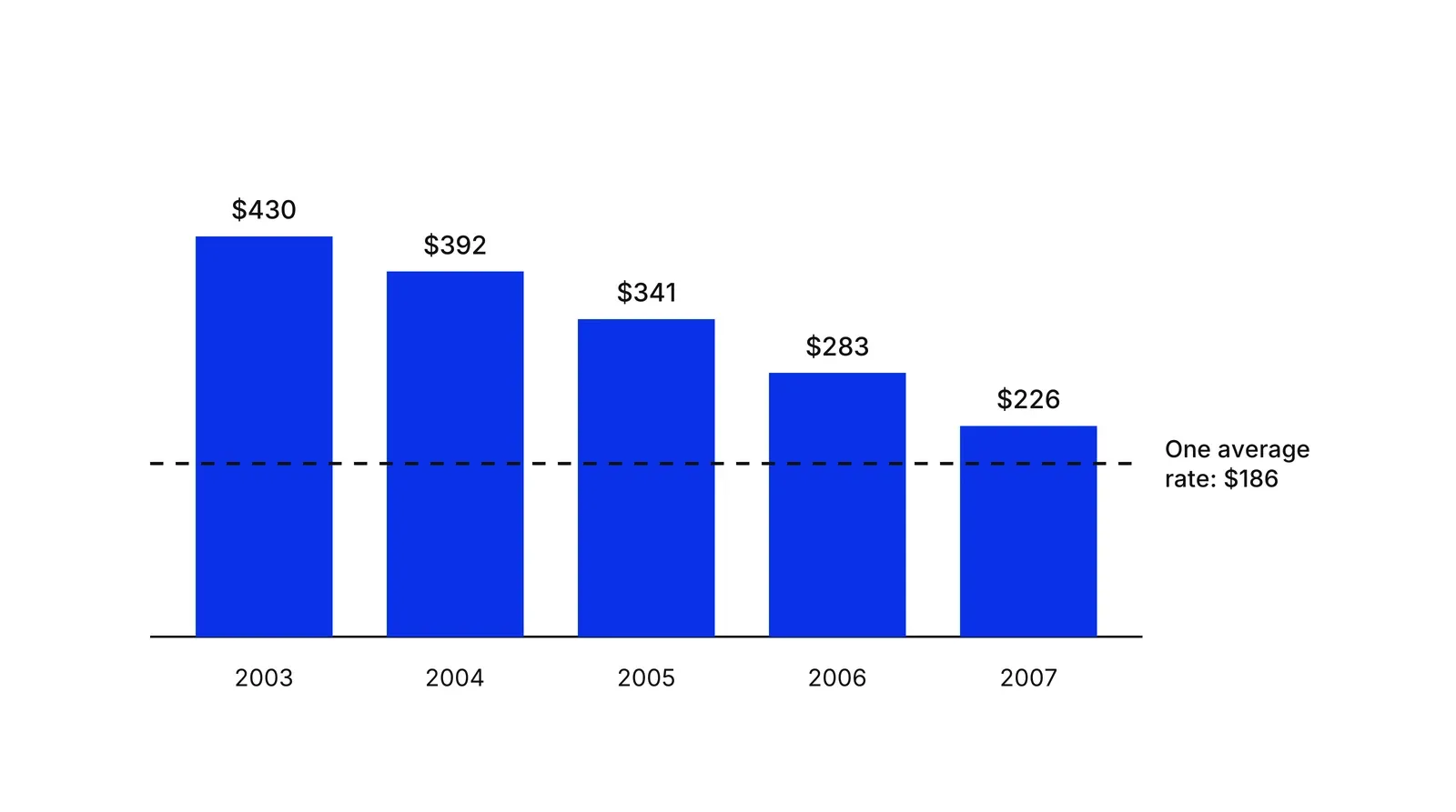
Five blue bars for the 2003 to 2007 acquisition cohorts showing expected residual value per customer of $430, $392, $341, $283 and $226, falling from left to right. A dashed black horizontal line at $186, labelled one average rate, runs below the tops of all five bars. — Every cohort is worth more than the single-rate figure, and the oldest cohorts are worth the most.

The per-cohort values follow from the paper’s own Bayes step: a customer who has renewed four times is 84% likely to belong to the loyal segment, and that probability is what lifts the value. The $186 line is the paper’s $4.95 million spread over its 26,569 active customers.

The pattern shows up in a listed company too. In McCarthy, Fader and Hardie’s valuation of Dish Network from public customer counts, the average customer was expected to stay about five and a half years, yet the model inferred a loyal segment of roughly 15% who stayed over a decade, as Knowledge at Wharton reports. Fader’s own advice is to speak of customers in the plural, because the average customer hides the spread.

The effect also works in the other direction for decisions. Fader and Hardie report that retention elasticities computed from a single rate understate the true effect of improving retention, which matters because Gupta and colleagues find that a 1% retention gain raises customer value by 3 to 7%, against 0.02 to 0.3% for the same gain in acquisition cost.

How do you build the cohort table?

Count customers by acquisition period and by age, and keep unfinished periods out of the denominator. A young cohort has not reached age 6 yet, so its age-6 cell stays empty rather than showing zero. Amplitude leaves intervals that have not finished out of the totals for this reason, and the Kaplan-Meier method described in the BMJ removes customers who have not yet had the chance to leave from later intervals. ChartMogul offers the table by month, quarter or year, with customer and net MRR retention. One caution from Knowledge at Wharton’s excerpt of Gupta and Lehmann: aggregate figures can hide wide gaps between customers, so check margin per cohort as well as counts.

How do you project the ages you have not seen?

You fit a model of how long customers stay and extend it, instead of drawing a line through the last few points. For subscriptions and other settings where leaving is visible, Fader and Hardie use the shifted beta-geometric model with two parameters, alpha and beta. Retention at age t is (beta + t - 1) divided by (alpha + beta + t - 1), so it rises with age by construction. They fitted it to seven years of data and tracked years eight to twelve closely; with the published parameters for the regular segment (0.704 and 1.182) the formula gives 62.7% retention in year one and 94.5% in year twelve. The same paper shows linear, quadratic and exponential fits missing year-twelve survival by large margins. A later 2018 study concludes that allowing for differences between customers matters more than allowing for changes within one customer over time. A spreadsheet version exists for teams without a statistician.

When leaving is not visible, the model has to infer it. A shop customer or a quiet merchant may have left or may be between purchases. The Pareto/NBD model of Schmittlein, Morrison and Colombo handles this, and the BG/NBD model gives similar results with far simpler estimation. The lifetimes Python library implements it from frequency, recency and age. RFM analysis supplies the same inputs, and the authors’ RFM and CLV paper links the two.

	Margin divided by churn	Cohort table, observed only	Cohort plus projection
Input	One churn rate	Counts by cohort and age	Counts by cohort and age, plus a model
Handles mixed customers	No	Yes, within the data window	Yes, beyond the window too
Weak spot	Understates value when retention rises	Ignores customers still alive at the end	Needs enough cohort history to fit
Fits	A first estimate	Payback and early value	Spend and valuation decisions

When is a single rate still good enough?

When retention at the cohort level does not rise. If each cohort loses the same share every period, the cohort is close to homogeneous and margin divided by churn is a fair summary. The single-rate formula also stays the common shortcut: Kellogg uses the inverse of annual churn and still warns that many distributions give the same average. Gurley adds that purchased and organic customers differ, which is a reason to build cohorts by channel as well as by month.

A cohort view also does not rescue a business with too little history. Tunguz argues that young companies cannot yet forecast lifetimes and should lean on payback, which you can read next to CAC payback period and the LTV:CAC ratio. The cohort table itself is built as in cohort analysis, and its plateau reading is covered in retention curves. Skok frames the first checks: are most customers lost in the first months, and does churn stabilize later.

A Growth Lab plan builds cohort LTV into the unit-economics review before any channel budget is raised: Growth Lab.

How to apply Cohort-based LTV, step by step

Define the cohort and what counts as active. Group customers by the month or quarter they were acquired, and write down the event that keeps them in the group: a renewed contract, a payment, a visit. Result: one sentence that decides who is in each cohort and who has left.
Build the table of active customers by age. For each cohort, count how many customers are still active at age 1, 2, 3 and so on, and leave empty the ages a young cohort has not reached yet. Result: a triangle of counts that gives the observed share still active at each age.
Read the retention rate between ages. Divide each age's count by the previous one. If the rate rises as cohorts age, a single average rate is understating the tail. Result: a view of whether the customer mix is sorting itself.
Project the missing ages. Extend the share still active beyond the data with a probability model, such as the shifted beta-geometric for subscriptions or BG/NBD for repeat purchases, rather than a straight line. Result: a share still active for every future period.
Multiply, discount and add. Multiply margin per active customer by the share still active, discount each period at your rate and sum over a horizon you can defend. Result: LTV per customer for each cohort.
Set it against acquisition cost by cohort. Compare each cohort's LTV with what it cost to acquire, by channel where you can, and refresh the projection each quarter as cohorts age. Result: a cohort-level ratio you can act on.

Examples

The published case behind the 38% gap

Illustrative, from Fader and Hardie's 2010 paper. A firm acquires 10,000 customers a year and earns $100 a year from each active one. One third of customers keep a constant 90% annual retention, two thirds keep 50%. The cohort shows 63.3%, 68.9%, 74.7% and 79.8% retention in successive years, though nobody changes behavior. One average rate of 69.1% values the customer base at about $4.95 million. The segment-aware answer is $7.94 million.

A dental membership plan

Illustrative arithmetic, no discounting. Members pay $40 a month and $24 is left after hygienist time and consumables. 40% of new members are short-stay and cancel at 20% a month; 60% are long-stay and cancel at 2% a month. First-month churn reads 9.2%, so the single-rate lifetime is 10.9 months and LTV $261. The true mean lifetime is 0.4 x 5 + 0.6 x 50 = 32 months, so LTV is $768.

A payments merchant with no cancel button

Illustrative. A merchant stops processing and never tells the provider, so the provider cannot see churn. That is the noncontractual case. The cohort table then counts merchants with at least one payment in each month, and the projection uses BG/NBD, which estimates the probability that a quiet merchant is still active from the frequency and recency of their payments.

When to use it

Use it when you buy customers with real money and have at least a few quarterly or annual cohorts: subscriptions, memberships, accounts, repeat-purchase businesses. It matters most when the answer feeds a spending decision, a channel comparison or a valuation, because those are the places where a flattering or a gloomy average does damage.

When not to use it

Skip the projection step for a company so young that no cohort has aged: there is no shape to extend, and a forecast from three data points is a guess with a formula around it. Skip it for one-off purchases with no repeat behavior. In both cases read observed payback first and add the model later.

Common mistakes

Applying the churn of the first month or the blended churn of all customers to the whole lifetime. Kellogg warns that many different distributions share the same average churn, and Fader and Hardie show that a rising cohort retention rate makes the single rate understate value.
Reading rising retention as customers growing loyal. In the shifted beta-geometric model every customer's own churn probability is constant, and the rise comes from quick leavers going first, the effect Vaupel and Yashin call the ruse of heterogeneity.
Pooling cohorts from different channels. Gurley points out that purchased customers tend to churn faster than organic ones, so a blended curve hides which spend creates value.
Straight-line extrapolation. Fader and Hardie's replication of a data-mining textbook case shows linear and quadratic fits breaking down well inside the 12 years of known data.
Counting only the observed months and calling it LTV. Fader and Hardie note that doing so ignores customers still alive at the end of the window and underestimates lifetime value.

FAQ

What is the formula for cohort-based LTV?

LTV is the sum over periods of margin times the share of the cohort still active, divided by one plus the discount rate to the power of the period. Fader and Hardie write it with the survivor function. The simple margin divided by churn formula is the special case of constant retention.

How do you calculate LTV in a bank?

Treat the account opening month as the cohort and count accounts still open or active at each age. Where customers can close an account, the setting is contractual and a retention model fits. Where they go quiet without closing, you need a rule for active and a repeat-buying model such as BG/NBD.

How is CAC used with cohort LTV?

LTV does not include CAC. Compute LTV per customer for each cohort, then divide by the acquisition cost of that cohort, ideally by channel. Skok's 3:1 guideline compares the two, and its reliability depends on how honest the lifetime behind LTV is.

How much cohort history do I need?

Enough to see whether retention levels off. Skok's cohort questions are whether most customers are lost in the first months and whether churn stabilizes later. If your oldest cohort has not reached a plateau, project cautiously and report a range, because Tunguz notes that young companies cannot yet forecast customer lifetimes.

Is cohort LTV the same as the simple LTV formula with segments?

No. Splitting customers into segments and averaging helps, but segments are often unobserved: Fader and Hardie's two groups are never labelled in the data. A cohort model infers the mix from how the observed retention curve bends, which works without knowing who belongs where.

Sources

Last updated Oct 9, 2026

Ilia PushinFounder, PUSHERS & COO Fintech ServiceIlia builds operating systems for growing companies in fintech and healthcare. Since 2021 he has run cross-border payments at ARBI Exchange, a licensed currency exchange in Thailand, including KYC and AML and the move into new jurisdictions.About the author LinkedIn

Related frameworks

More frameworks

Related insights

Three cylinders on a white marble slab, growing from short to tall: two in polished chrome, the tallest in frosted glass, on a light grey background.

Growth systemsArticle

Marketing agency or growth system: when a company outgrows its agency

An agency is the right call while the founder still runs most of the company. Once the business starts copying itself into new locations or markets, it needs a system that sets goals, tests hypotheses and owns the result.

Oct 7, 2026 · 7 min read

Three frosted-glass blocks rising in height like steps, with a small blue sphere on the lowest one, on a light grey background.

Growth systemsArticle

Why healthcare marketing agencies stall: the short, mid and long wins model we use with clinics

Most agencies own the click and nobody owns the front desk. How we structure clinic work in three horizons, the research behind each one, and one year of results.

Sep 26, 2026 · 9 min read

A stack of chrome coins beside a glass hourglass on a light grey background.

Finance operationsPlaybook

How to calculate channel payback and unit economics

A CAC number that only marketing believes will not survive a finance review. This guide calculates channel payback so both teams work from the same model.

Sep 23, 2026 · 7 min read

Want Cohort-based LTV running inside your company?Request an operations audit