Statistical significance
Statistical significance is a verdict that a measured difference is too large to be easily explained by chance alone, usually because its p-value falls below a threshold set in advance, most often 0.05.
Statistical significance means a measured difference, such as a higher conversion rate in variant B, would be unusual if there were no real difference between the variants. It is usually declared when the p-value falls below a threshold chosen before the test, most often 0.05. It says nothing about the size or business value of the difference, nor the chance that the result is true.
- Origin
- Ronald A. Fisher (significance tests); Jerzy Neyman and Egon Pearson (error rates and decision rules), 1925; from 1928
- Level
- 201 · Tool
- Fits
- Small and mid-size, Scale-up
- Time to apply
- 30 minutes to write a decision rule before the next test
- What you need
- a test with a primary metric and a planned sample size · a threshold for the smallest lift that would change a decision · the raw counts from both variants, not just the dashboard verdict
Statistical significance is a label for a result that would be unusual if there were no real difference. In an A/B test, you assume the variants perform the same, then ask how often chance alone would produce a gap at least as large as the one you saw. If that share, the p-value, falls below a threshold fixed in advance, usually 5%, the result is called significant. The label answers one narrow question, and most misuse comes from asking it to answer three others: how big the effect is, whether it matters, and whether it is true.
Where did the 0.05 line come from?
The 5% line is a convention, and it comes from two schools that were later blended. In Statistical Methods for Research Workers (1925), Ronald Fisher showed that a deviation of about two standard deviations leaves 1 chance in 20 and wrote that it is “convenient to take this point as a limit”. For Fisher the p-value was a measure of evidence against the null hypothesis, the assumption of no difference.
Jerzy Neyman and Egon Pearson, from 1928 onward, built a different method. It fixes a significance level (alpha) and a power in advance, names an alternative hypothesis and treats the test as a decision rule with known long-run error rates. José Perezgonzalez’s 2015 tutorial lays out the two approaches and calls today’s null hypothesis significance testing (NHST) an amalgam of them.
| Fisher | Neyman and Pearson | Typical A/B practice | |
|---|---|---|---|
| Role of the p-value | Evidence against the null | Compared with a preset alpha | Both, often confused |
| Alternative hypothesis | Implicit only | Explicit, with an effect size | Often skipped |
| Power | Not used | Planned in advance | Planned, if the team sizes tests |
| Output | A graded strength of evidence | Reject or do not reject | A green or red badge |
What a p-value says, and what it does not
A p-value is the probability of seeing data at least as extreme as yours if the null hypothesis, and every other assumption of the model, were true. Statsig’s documentation puts it as how surprising your result would be if the treatment did nothing.
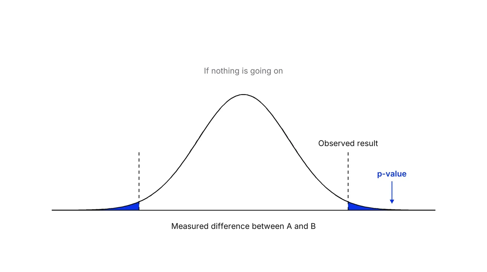
In March 2016 the American Statistical Association issued a statement on p-values, the first time its board had addressed these issues. Its six principles include that p-values do not measure the probability the hypothesis is true, that decisions should not rest only on whether a p-value passes a threshold, and that a p-value does not measure effect size or importance. Sander Greenland and colleagues list 25 misreadings. Their first is the belief that the p-value is the probability that the test hypothesis is true.
So p = 0.03 does not mean a 97% chance that variant B is better. Some tools do report a probability that B beats A, such as GrowthBook’s chance to win, but it comes from a Bayesian model, which the sequential and Bayesian testing page covers.
Significant is not the same as worth shipping
A significant result tells you an effect probably exists. It does not tell you the effect is large enough to act on. Statsig’s guidance is to use the p-value to decide whether an effect exists and the confidence interval to judge how large it is. Kohavi and colleagues likewise recommend reporting a confidence interval for the effect next to the test result.
The figure below uses the arithmetic of three illustrative tests of a checkout page with 5% baseline conversion, against an assumed smallest lift worth shipping of 0.2 points.
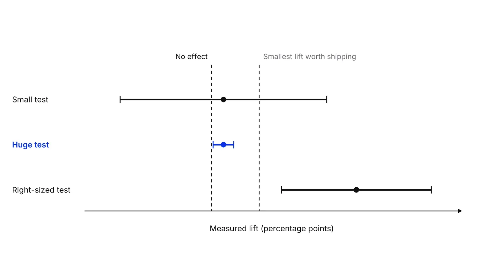
The small test (20,000 users per variant, 5.00% against 5.05%) has p = 0.82 and an interval of -0.38 to +0.48 points. It cannot rule out a useful lift or a loss. The huge test (2,000,000 per variant, same observed gap) has p = 0.022 and an interval of 0.007 to 0.093 points. It is significant and still too small to matter. A right-sized test (40,000 per variant, 5.0% against 5.6%) has p = 0.0002 and an interval of 0.29 to 0.91 points, clear of both lines. Planning the size of a test around the smallest lift that matters is the subject of the minimum detectable effect and sample size page.
How often is a significant result wrong?
More often than 5%, because 5% describes tests of ideas that do nothing, and no one knows how many of their ideas are in that group. The false positive rate among significant results depends on the share of tested ideas that are real. The formula, given by Benjamin and colleagues, is alpha x share of true nulls, divided by that same term plus power x share of real effects. Our calculation, at 80% power:
| Share of tested ideas that are real | Wrong among significant results at 0.05 | At 0.005 |
|---|---|---|
| 50% | 5.9% | 0.6% |
| 20% | 20% | 2.4% |
| 10% | 36% | 5.3% |
Benjamin and colleagues reach the same place, with a false positive rate above 33% at prior odds of 1:10, and propose moving the default for new discoveries to 0.005, calling results between 0.005 and 0.05 “suggestive”. The price is samples about 70% larger at the same power. David Colquhoun argued from several angles that p = 0.05 gives a false discovery rate of at least 30%. John Ioannidis made the general case in 2005 that small samples, small effects and many tested relationships push findings toward false.
Not everyone accepts a new universal cutoff. A large group of researchers answered in the same journal with “Justify your alpha”, and a 2019 Nature comment by Amrhein, Greenland and McShane, backed by more than 800 signatories, called for an end to hyped claims and to the dismissal of effects that may matter. For a growth team the lesson is practical: pick the alpha by the cost of being wrong, write it down before launch, and keep a log of past tests so you know your own share of real wins, as the experimentation program page describes.
Many metrics, many segments, many looks
Every extra comparison is another chance for noise to cross the line. With 20 independent comparisons at 5%, the chance of at least one false hit is 1 - 0.95^20, or 64% (our arithmetic). Simmons, Nelson and Simonsohn showed in 2011 that flexibility in what to measure and when to stop can make a false positive more likely than not. Controlling the false discovery rate, as in Benjamini and Hochberg’s 1995 method, is one remedy. Naming one primary metric before launch is a simpler one. Checking a running test repeatedly breaks the guarantee for a similar reason, which Johari, Pekelis and Walsh address with always valid p-values.
Two further traps are common. Gelman and Stern pointed out that the difference between “significant” and “not significant” is not itself significant, so a segment that crosses 0.05 beside one that does not proves nothing about the gap between them. And a result that looks too good deserves suspicion: Kohavi and Thomke describe a Bing headline test that raised revenue by 12% and tripped a “too good to be true” alert. Kohavi’s team also recommends continuous A/A tests, which should come out non-significant 95% of the time, and a check that users are split in the planned proportions.
What to report instead of a badge
Report the estimate, its interval and the decision, with the p-value as one input. The 2019 editorial in The American Statistician by Wasserstein, Schirm and Lazar went further and urged researchers to stop using the phrase “statistically significant” altogether. In a business setting the same advice becomes a habit: a test summary that says “+0.6 points, interval 0.29 to 0.91, p = 0.0002, ship” carries more than a green tick. A Growth Lab plan starts from a written decision rule like this one, set before the first test.
How to apply Statistical significance, step by step
- Write the decision rule before launch. Fix the significance level (usually 5%), the primary metric and the smallest lift worth shipping, then size the test for that lift. Result: one sentence that says what outcome means ship, stop or rerun.
- Check the test is healthy. Confirm that traffic was split in the planned proportions and that the setup passes an A/A test, which should show a significant difference about 5% of the time. Result: a yes or no on whether the numbers can be trusted at all.
- Read the interval, not only the p-value. Take the confidence interval for the difference and compare its whole width with the smallest lift worth shipping. Result: a range of plausible effects instead of a pass or fail stamp.
- Count what you compared. List every metric, segment and look at the data that fed the decision. If you checked 20 segments, expect a false hit among them. Result: the true number of comparisons, with a stricter threshold or a clearly labelled hypothesis for anything beyond the primary metric.
- Write the verdict in three parts. State the estimate with its interval, the p-value and the decision. Add what would change your mind. Result: a one-paragraph record that goes into the experiment log.
Examples
A clinic's online booking button
Illustrative. A dental clinic tests a new booking button on 20,000 visitors per variant. Booking rates are 5.00% and 5.05%, p = 0.82, and the interval for the lift runs from -0.38 to +0.48 points. The test is not significant, but it is also too small to show anything: the interval still allows a lift worth having. The decision is to rerun with a sample sized for the smallest useful lift.
A payments checkout with a huge test
Illustrative. A payments product tests a checkout change on 2,000,000 users per variant. Conversion moves from 5.00% to 5.05%, p = 0.022, so the result is significant, and the interval runs from 0.007 to 0.093 points. If the team decided that anything under 0.2 points is not worth the engineering time, significance does not change the decision.
A segment report on a SaaS trial
Illustrative. A team slices one test by 20 segments and finds one with p = 0.03. With 20 independent comparisons at a 5% threshold, the chance of at least one false hit is 64%. The segment becomes a hypothesis for the next test, not a result.
When to use it
Use significance testing when you run a controlled experiment with a planned sample, a primary metric and a decision that depends on telling a real change from noise. It is a good guard against acting on random swings in conversion or revenue.
When not to use it
Do not use a p-value as the only basis for a business decision, to rank many ideas that were mined from the data after the fact, or to prove that two options are the same. A non-significant result in a small test shows that the test was too weak, not that nothing happened.
Common mistakes
- Reading p = 0.03 as a 97% chance that the variant is better. The p-value is computed assuming there is no real difference, so it cannot give the probability of the variant being better.
- Treating significance as importance. With enough traffic, a trivial change becomes significant.
- Taking a non-significant result as proof of no effect, and then dropping the idea.
- Slicing the result by many segments or metrics after the fact and reporting the one that crossed 0.05.
- Comparing two segments by noting that one is significant and the other is not, when the difference between them was never tested.
FAQ
What is a good level of statistical significance?
The common default is 5% (p below 0.05), but it is a convention, not a law. Fisher called it convenient in 1925. A product team should set the level before the test according to the cost of a wrong call: stricter for a costly or hard-to-reverse change, looser for a cheap, reversible one.
Does p = 0.05 mean I am 95% sure the result is real?
No. The American Statistical Association says p-values do not measure the probability that the studied hypothesis is true. A p-value of 0.05 says the data would be unusual if there were no effect. The chance the result is real also depends on how plausible the idea was before the test.
What is the difference between statistical and practical significance?
Statistical significance says a difference is unlikely to be pure chance. Practical significance asks whether it is big enough to matter for revenue, cost or risk. A huge sample can make a tiny lift significant, so compare the confidence interval with the smallest lift worth acting on.
How do I test the statistical significance of a difference between two variants?
Compare the two rates with a two-sample test, such as a z-test for conversion rates or a t-test for averages. Report the difference, its confidence interval and the p-value. Plan the sample size first and run the test to that size, because peeking inflates false positives.
Sources
- American Statistical Association, ASA releases statement on statistical significance and p-values, March 2016
- Ronald L. Wasserstein, Allen L. Schirm, Nicole A. Lazar, Moving to a world beyond p < 0.05, The American Statistician 73(S1), 2019
- Ronald A. Fisher, Statistical Methods for Research Workers, chapter III, 1925 (Classics in the History of Psychology)
- Jose D. Perezgonzalez, Fisher, Neyman-Pearson or NHST? A tutorial for teaching data testing, Frontiers in Psychology 6, 2015
- Daniel J. Benjamin et al., Redefine statistical significance, Nature Human Behaviour 2, 2018
- Daniel Lakens et al., Justify your alpha, Nature Human Behaviour 2, 2018
- Sander Greenland et al., Statistical tests, P values, confidence intervals, and power: a guide to misinterpretations, European Journal of Epidemiology 31, 2016
- John P. A. Ioannidis, Why Most Published Research Findings Are False, PLoS Medicine 2(8), 2005
- David Colquhoun, An investigation of the false discovery rate and the misinterpretation of P values, arXiv 1407.5296, 2014
- Valentin Amrhein, Sander Greenland, Blake McShane, Scientists rise up against statistical significance, Nature, March 2019
- Regina Nuzzo, Scientific method: statistical errors, Nature 506, 2014
- Joseph P. Simmons, Leif D. Nelson, Uri Simonsohn, False-positive psychology, Psychological Science 22(11), 2011
- Yoav Benjamini, Yosef Hochberg, Controlling the false discovery rate, Journal of the Royal Statistical Society B 57(1), 1995
- Andrew Gelman, Hal Stern, The difference between significant and not significant is not itself statistically significant, The American Statistician 60(4), 2006
- Ron Kohavi, Roger Longbotham, Dan Sommerfield, Randal M. Henne, Controlled experiments on the web: survey and practical guide, Data Mining and Knowledge Discovery 18, 2009
- Ron Kohavi, Stefan Thomke, The surprising power of online experiments, Harvard Business Review, September-October 2017
- Ron Kohavi, Diane Tang, Ya Xu, Trustworthy Online Controlled Experiments, Cambridge University Press, 2020
- Ramesh Johari, Leo Pekelis, David J. Walsh, Always valid inference: bringing sequential analysis to A/B testing, arXiv 1512.04922
- Statsig documentation, P-value
- GrowthBook documentation, Statistics overview
Last updated Oct 9, 2026


Marketing agency or growth system: when a company outgrows its agency
An agency is the right call while the founder still runs most of the company. Once the business starts copying itself into new locations or markets, it needs a system that sets goals, tests hypotheses and owns the result.

Why healthcare marketing agencies stall: the short, mid and long wins model we use with clinics
Most agencies own the click and nobody owns the front desk. How we structure clinic work in three horizons, the research behind each one, and one year of results.

Why channel tests stall after month three
Most paid channel tests do not end with a decision. They end when the budget runs out, the attribution model changes, or everyone quietly stops looking at the dashboard.