Forecasting and time series

Origin

Charles Holt, Peter Winters, George Box and Gwilym Jenkins, Cleveland and colleagues, Sean Taylor and Ben Letham, Holt 1957; Winters 1960; Box and Jenkins 1970; STL 1990; Prophet 2018

Level

401 · Expert

Fits

Scale-up, Enterprise

Time to apply

One day for a first benchmark and a rolling test on one metric

What you need

a regular series of at least two or three years of the metric, one value per day, week or month · a list of known events that distort it: promotions, price changes, outages, holidays · one person who owns the forecast and will log it before the period starts

Time series forecasting is the practice of predicting a metric’s future values from its own history: weekly orders, monthly bookings, daily transactions. This page covers the statistical toolkit for that job. For the pipeline-based and judgmental ways to forecast revenue, see sales forecasting methods; the two fit together, and the error measures below apply to both.

Can this metric be forecast at all?

A metric is forecastable to the degree that four things hold, according to Rob Hyndman and George Athanasopoulos in Forecasting: Principles and Practice: you understand its drivers, you have enough data, the future resembles the past, and the forecast does not change the thing being forecast. Short-term household electricity demand passes all four, since temperature drives it. Exchange rates fail most of them, because crises break past patterns and published forecasts can move the rate, and the book calls predicting a rise or fall about as predictable as a coin toss.

Business metrics sit between. Run the check first; it decides whether to build a model or use scenario planning.

Decomposition: trend, seasonality, remainder

Decomposition splits a series into a slow trend, a repeating seasonal pattern and a remainder. Classical decomposition, which dates to the 1920s, averages each season across years. The textbook now advises against it: it assumes the seasonal pattern never changes and reacts badly to unusual values.

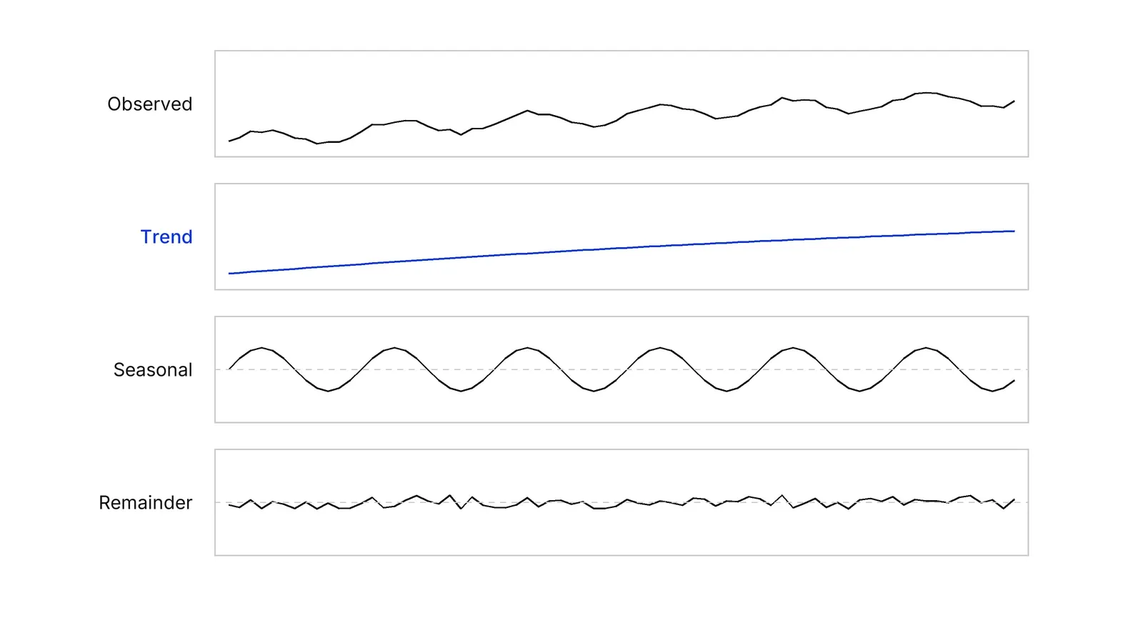
STL, short for seasonal and trend decomposition using loess, was published by Robert Cleveland, William Cleveland, Jean McRae and Irma Terpenning in the Journal of Official Statistics in 1990. The textbook lists its advantages: the seasonal pattern can change over time, any seasonal period works, and an option limits the pull of outliers. The defaults use a seasonal window of 11 and, for monthly data, a trend window of 21 observations; smaller windows let the pattern change faster. Plot the parts to spot a level shift or promotion spike before modelling.

Exponential smoothing and the ETS family

Exponential smoothing forecasts with a weighted average of past values in which recent values weigh most. Holt extended it to trends in 1957 and Winters to seasonality in 1960, and the Holt-Winters method keeps three smoothed pieces: level, trend and seasonal pattern. Use the additive form when seasonal swings stay about the same size and the multiplicative form when they grow with the level. The book reports that a damped trend with multiplicative seasonality often gives accurate forecasts for seasonal data.

The ETS framework writes each variant as a model with an Error, a Trend and a Seasonal part, which gives prediction intervals and lets software pick among models by an information criterion. The forecast package paper describes automatic fitting of both ETS and ARIMA across many series.

ARIMA: modelling the autocorrelation

ARIMA models forecast from a series’ own past values and past forecast errors, after differencing turns it into a stationary series. A stationary series has statistical properties that do not depend on when you look; trends and seasonality break that, and differencing, which replaces each value with its change from the last, removes them. A seasonal difference subtracts the value from the same month last year, and the textbook’s rule of thumb recommends one when seasonal strength is at least 0.64. The approach comes from George Box and Gwilym Jenkins, whose book is now in its fifth edition.

The Hyndman-Khandakar algorithm automates the choice: repeated KPSS tests set the number of differences (0, 1 or 2), a p-value below 0.05 signalling that differencing is needed, then a stepwise search lowers the AICc. ETS and ARIMA overlap but neither contains the other, and AICc cannot compare across the two families, so use cross-validation for that. The textbook’s examples show why: on Australian population, a non-seasonal series, ETS had a cross-validated RMSE of about 0.077 against 0.194 for ARIMA, while on seasonal cement production ARIMA edged ahead on a test set, 216 to 222.

Prophet: trend, seasonality and holidays for analysts

Prophet is a forecasting tool that adds a flexible trend, seasonal cycles and a holiday table. Sean Taylor and Ben Letham describe it as built for many business series and too few forecasting specialists, pairing a model with interpretable settings an analyst can adjust. Its input is two columns: a date and a value.

It looks for trend changes at 25 candidate changepoints in the first 80% of the history, keeping few through a sparse prior whose default strength is 0.05. Seasonality uses Fourier terms, with defaults of order 10 for yearly and 3 for weekly patterns; holidays come from a table you supply, with a default prior scale of 10; extra regressors need future values. Marketing mix models extend the idea with spend as regressors.

Method	Best for
Seasonal naive	The benchmark every model must beat
ETS	Clear trend and seasonality, automatic fitting
ARIMA	Series with autocorrelation after differencing
Prophet	Daily data, several cycles, holidays, trend breaks

How do you score a forecast?

Score a forecast on data the model never saw, using time series cross-validation: each test point is forecast from only the observations before it, and the origin rolls forward. Prophet’s diagnostics do the same, with an initial window of three times the horizon and a cutoff every half horizon by default.

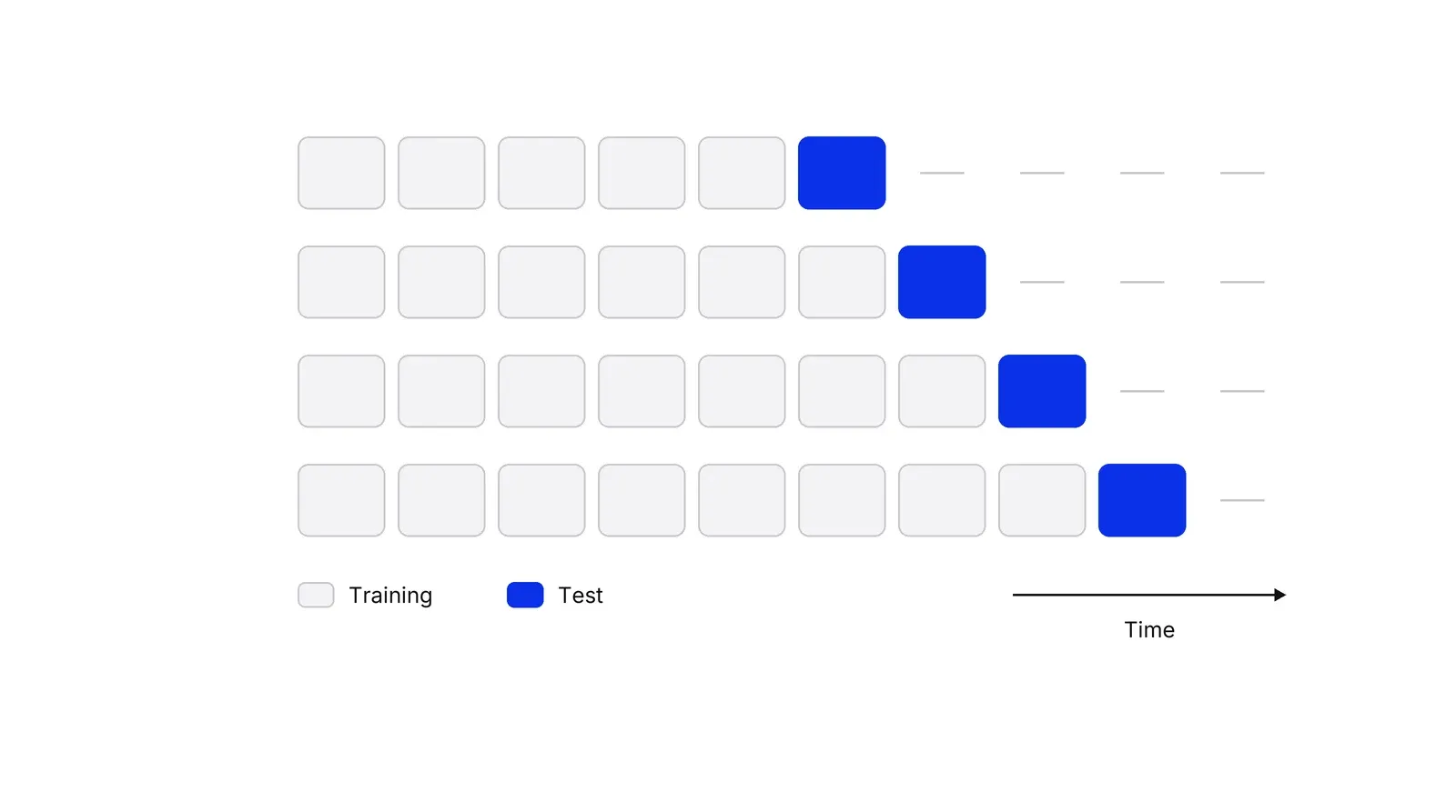
Then pick the measure. MAE and RMSE are in the data’s units. MAPE is a percentage, but it is undefined when an actual is zero. Rob Hyndman and Anne Koehler proposed the mean absolute scaled error after finding that older measures are often undefined or misleading. MASE divides the error by the in-sample error of a naive forecast, so below one beats naive. Take an illustrative clinic whose seasonal naive forecast has an in-sample MAE of 50 bookings a month. Dividing each model’s rolling-origin MAE by 50 gives its MASE:

Method	MAE (bookings)	MASE	Beats naive?
Seasonal naive	50	1.00	Baseline
ETS	38	0.76	Yes
ARIMA	41	0.82	Yes
Prophet	53	1.06	No

Track the signed average error too, to catch bias.

Show a range with the number. A prediction interval widens as the horizon grows, and 80% and 95% are the usual levels, with multipliers of 1.28 and 1.96 on the forecast standard deviation if errors are normal. A forecast of 420 bookings with a standard deviation of 30 gives an 80% interval of 382 to 458 and a 95% interval of 361 to 479. When two models differ by a small margin over a few origins, treat the gap with the care that statistical significance asks of an A/B test.

What do the M-competitions say?

The M-competitions are open contests run by Spyros Makridakis and colleagues, with Michele Hibon on M3 and Evangelos Spiliotis and Vassilios Assimakopoulos on M4 and M5, in which teams forecast the same series and are scored on held-out data. Three results shape practice. In 2018, Makridakis and colleagues found that popular machine learning methods were dominated by eight statistical ones on 1,045 monthly series from the M3 competition. In M4, 12 of the 17 most accurate methods were combinations of mostly statistical approaches, and the six pure machine learning methods performed poorly: none beat the combination benchmark. A hybrid of statistical and machine learning features was the biggest surprise, with an average sMAPE close to 10% better than that benchmark.

M5 changed the picture for retail: on 42,840 Walmart unit-sales series, only 415 teams, 7.5% of the field, beat the best statistical benchmark, and the five winners beat it by more than 20%, mostly with LightGBM models. The first-place entry came from YeonJun Im, a senior undergraduate, and 48.4% of all teams beat the simple Naive benchmark. The earlier M3 and M4 winners had beaten their benchmarks by less than 10%. The lesson is about data: thousands of related series with prices and events reward machine learning; one short series rewards simple methods and a good benchmark.

Where does it fit?

Statistical forecasts feed the financial model for growth as the baseline that scenarios then move up or down. Known drivers can enter as regressors, as regression with time series shows. A Growth Lab plan starts from the forecast error history, because a target set on an unscored forecast is a guess.

How to apply Forecasting and time series, step by step

1. Check the metric can be forecast. Ask the four questions in the first section below: are the drivers understood, is there enough history, will the future resemble the past, does the forecast change the outcome? Result: a yes or no on a statistical forecast, and a list of what breaks the pattern.
2. Plot the series and decompose it. Split the series into trend, seasonal pattern and remainder with STL. Note the seasonal period (12 for monthly data, 7 for daily), outliers and level shifts. Result: a clear read of trend and seasonal size before any model is chosen.
3. Set the benchmarks. Forecast with the naive method and the seasonal naive method, which repeats the same period last year. Every later model has to beat both. Result: two error numbers a complex model must improve on.
4. Fit two or three candidates. Fit ETS and ARIMA and, if holidays or several seasonal cycles matter, Prophet. Add known events as inputs where future values are known. Result: three forecast sets for the same periods.
5. Score on a rolling origin. Move the origin forward through the last 12 to 24 periods, forecast the horizon you need each time, and compute MASE and bias at that horizon. Result: an error table per method and horizon, on unseen data.
6. Publish a range and log it. Show the point forecast with an 80% or 95% prediction interval, record each forecast before its period starts, and re-score monthly. Result: a forecast with a range and a running error record.

Examples

A dental clinic planning chair capacity

Illustrative. A clinic has 36 months of appointment counts with a dip each August and a rise each January. STL separates a slow upward trend from a seasonal swing of about 15%. The seasonal naive forecast is the benchmark; ETS and ARIMA are scored on 12 rolling origins at a 3-month horizon. The better one, with its 80% interval, sets hygienist rosters a quarter ahead.

A payments company forecasting transaction volume

Illustrative. Daily transaction counts have a weekly cycle, a yearly cycle, month-end peaks and national holidays. Prophet takes a holiday table and handles both cycles directly; ARIMA needs more manual setup. Both are scored against the seasonal naive benchmark on a 28-day horizon. A new payout corridor is a level shift, so it goes in as a known event and its first 4 weeks get manual review.

When to use it

Use it when a metric has a regular history and you must plan on it: capacity, stock, cash, staffing, ad budget pacing. It suits seasonal series with a stable business behind them.

When not to use it

Skip it when history is short or the business just changed: a new product, price list or market breaks the link between past and future. Skip it too when the forecast changes the outcome, as a sales target does.

Common mistakes

• Scoring the model on the data it was fitted to. Fitted error is always smaller than error on new data. Use a rolling forecasting origin.
• Skipping the benchmark. A model that cannot beat the seasonal naive forecast adds cost and no accuracy.
• Reporting only MAPE. It is undefined at a zero actual and treats over- and under-forecasts unevenly. Add MASE and the signed bias.
• Showing one number. Without an 80% or 95% prediction interval the reader cannot tell a firm forecast from a guess.

FAQ

Which time series forecasting method is best?

None wins everywhere. In the M4 competition, combinations of mostly statistical methods took 12 of the top 17 places and pure machine learning did poorly. In M5, on 42,840 related retail series, machine learning won. Start with a seasonal naive benchmark, then test ETS, ARIMA and one more method on your own data.

What is the difference between ARIMA and exponential smoothing?

Exponential smoothing describes level, trend and seasonality with weighted averages. ARIMA models the autocorrelation left after differencing makes the series stationary. The two overlap but neither contains the other, so compare them with cross-validation, not AICc, which only works within one family.

How do you measure forecast accuracy?

Compute errors on unseen data with a rolling forecasting origin. MAE and RMSE are in the data's units. MAPE is a percentage but breaks near zero. MASE scales the error by a naive forecast's in-sample error, so below 1 beats naive. Also track the signed bias.

How much history do I need to forecast?

Enough to show each seasonal cycle you model more than once. Prophet's documentation says the first training window should cover at least a year when you want yearly seasonality. A series of a few dozen points, common in B2B sales, usually supports only simple methods.

Sources

1. Rob J Hyndman, George Athanasopoulos, Forecasting: Principles and Practice (3rd ed.), What can be forecast?
2. Hyndman, Athanasopoulos, Forecasting: Principles and Practice, Classical decomposition
3. Hyndman, Athanasopoulos, Forecasting: Principles and Practice, STL decomposition
4. Hyndman, Athanasopoulos, Forecasting: Principles and Practice, Holt-Winters' seasonal method
5. Hyndman, Athanasopoulos, Forecasting: Principles and Practice, Innovations state space models for exponential smoothing
6. Hyndman, Athanasopoulos, Forecasting: Principles and Practice, Stationarity and differencing
7. Hyndman, Athanasopoulos, Forecasting: Principles and Practice, ARIMA models
8. Hyndman, Athanasopoulos, Forecasting: Principles and Practice, ARIMA modelling in fable
9. Hyndman, Athanasopoulos, Forecasting: Principles and Practice, ARIMA vs ETS
10. Hyndman, Athanasopoulos, Forecasting: Principles and Practice, Time series cross-validation
11. Hyndman, Athanasopoulos, Forecasting: Principles and Practice, Evaluating point forecast accuracy
12. Hyndman, Athanasopoulos, Forecasting: Principles and Practice, Some simple forecasting methods
13. Hyndman, Athanasopoulos, Forecasting: Principles and Practice, Prediction intervals
14. Hyndman, Athanasopoulos, Forecasting: Principles and Practice, Introduction to regression with time series
15. Robert B. Cleveland, William S. Cleveland, Jean E. McRae, Irma Terpenning, STL: A seasonal-trend decomposition procedure based on loess, Journal of Official Statistics 6(1), 1990
16. Rob J Hyndman, Yeasmin Khandakar, Automatic time series forecasting: the forecast package for R, Journal of Statistical Software 27(3), 2008
17. Wiley, Box, Jenkins, Reinsel, Ljung, Time Series Analysis: Forecasting and Control, 5th edition
18. Rob J Hyndman, Anne B Koehler, Another look at measures of forecast accuracy, International Journal of Forecasting 22(4), 2006
19. Sean J. Taylor, Benjamin Letham, Forecasting at scale, The American Statistician 72(1), 2018, Meta Research page
20. Prophet documentation, Quick start
21. Prophet documentation, Trend changepoints
22. Prophet documentation, Seasonality, holiday effects, and regressors
23. Prophet documentation, Diagnostics
24. Spyros Makridakis, Michele Hibon, The M3-Competition: results, conclusions and implications, International Journal of Forecasting 16(4), 2000
25. Makridakis, Spiliotis, Assimakopoulos, Statistical and Machine Learning forecasting methods: concerns and ways forward, PLOS ONE 13(3), 2018
26. Makridakis, Spiliotis, Assimakopoulos, The M4 Competition: results, findings, conclusion and way forward, International Journal of Forecasting 34(4), 2018
27. Makridakis, Spiliotis, Assimakopoulos, M5 accuracy competition: results, findings, and conclusions, International Journal of Forecasting 38(4), 2022
28. Makridakis, Spiliotis, Assimakopoulos, M5 accuracy competition, preprint with full results

Last updated Oct 9, 2026