Conjoint analysis

Origin

R. Duncan Luce and John Tukey (measurement theory); Paul E. Green and Vithala R. Rao (marketing); Jordan Louviere and George Woodworth (choice-based), 1964; 1971; 1983

Level

301 · Advanced

Fits

Scale-up, Enterprise

Time to apply

4 to 8 weeks for a first study: one to two weeks of qualitative work, a week of design and testing, two weeks in field, one to two weeks of analysis

What you need

a pricing or product decision with two to four real options on the table · qualitative interviews that tell you which attributes buyers weigh · access to 300 or more respondents from the target market · survey software that supports choice-based conjoint and an analyst who can read a logit model

Conjoint analysis is a survey experiment that measures how buyers trade one feature against another and against price. Instead of asking people what they value, it shows them complete offers, each built from a planned mix of features, and watches what they pick. A model then works backwards from those choices to a score for every feature level, called a part-worth.

The method has two roots. The mathematics is conjoint measurement, set out by R. Duncan Luce and John Tukey in 1964. Paul Green of Wharton saw the marketing use: according to Wharton Magazine, he came up with the idea and the name around 1964, and his 1971 paper with Vithala Rao in the Journal of Marketing Research introduced it to the field. In that first paper, as John Hauser recounts, one homemaker ranked all 36 possible profiles built from three features. Thirty years later Green, Abba Krieger and Yoram Wind called it marketers’ favorite methodology for studying trade-offs, with thousands of applications behind it.

Why ask for choices instead of ratings?

Because people say everything matters. Ask a shop owner to rate fee, payout speed and support on a 1 to 10 scale and all three get an 8. Make them choose between a cheap plan with slow payouts and a dearer plan with fast ones, and the real priority shows.

Early conjoint studies used rankings and ratings of profiles. In 1983 Jordan Louviere and George Woodworth combined conjoint with discrete choice models from econometrics, which gave rise to choice-based conjoint (CBC). Respondents see a few profiles at a time and pick one, or pick None if nothing appeals. Joel Huber’s history of the method records the shift from ratings back to choices, and Sawtooth Software’s 2019 user survey found CBC was the most used variant by a wide margin.

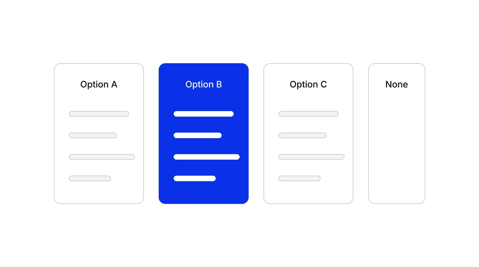
How a study is built

A conjoint study rests on three parts.

Attributes and levels come first. An attribute is a feature the buyer weighs, such as monthly fee; a level is one value of it, such as $15. They come from interviews, not from the product roadmap. Levels must be realistic, because a profile nobody would believe teaches the model nothing.

The experimental design decides which profiles appear together. Software builds a fractional design so that every level shows up about equally often and attributes vary independently. Each respondent answers a series of such tasks. Sawtooth Software’s sample size guidance suggests 300 respondents, 200 per reported subgroup, and at least 500 appearances of each level across the sample.

Estimation turns the choices into part-worths. A multinomial logit model gives average part-worths for the sample. Hierarchical Bayes, introduced to conjoint by Lenk, DeSarbo, Green and Young in 1996, estimates part-worths for each respondent from fewer tasks, which makes segmentation possible.

Part-worths and importance

A part-worth is the utility a level adds to an offer, on a scale shared by all attributes. Add the part-worths of an offer’s levels and you get its total utility. Compare total utilities and you can predict which offer a respondent would pick.

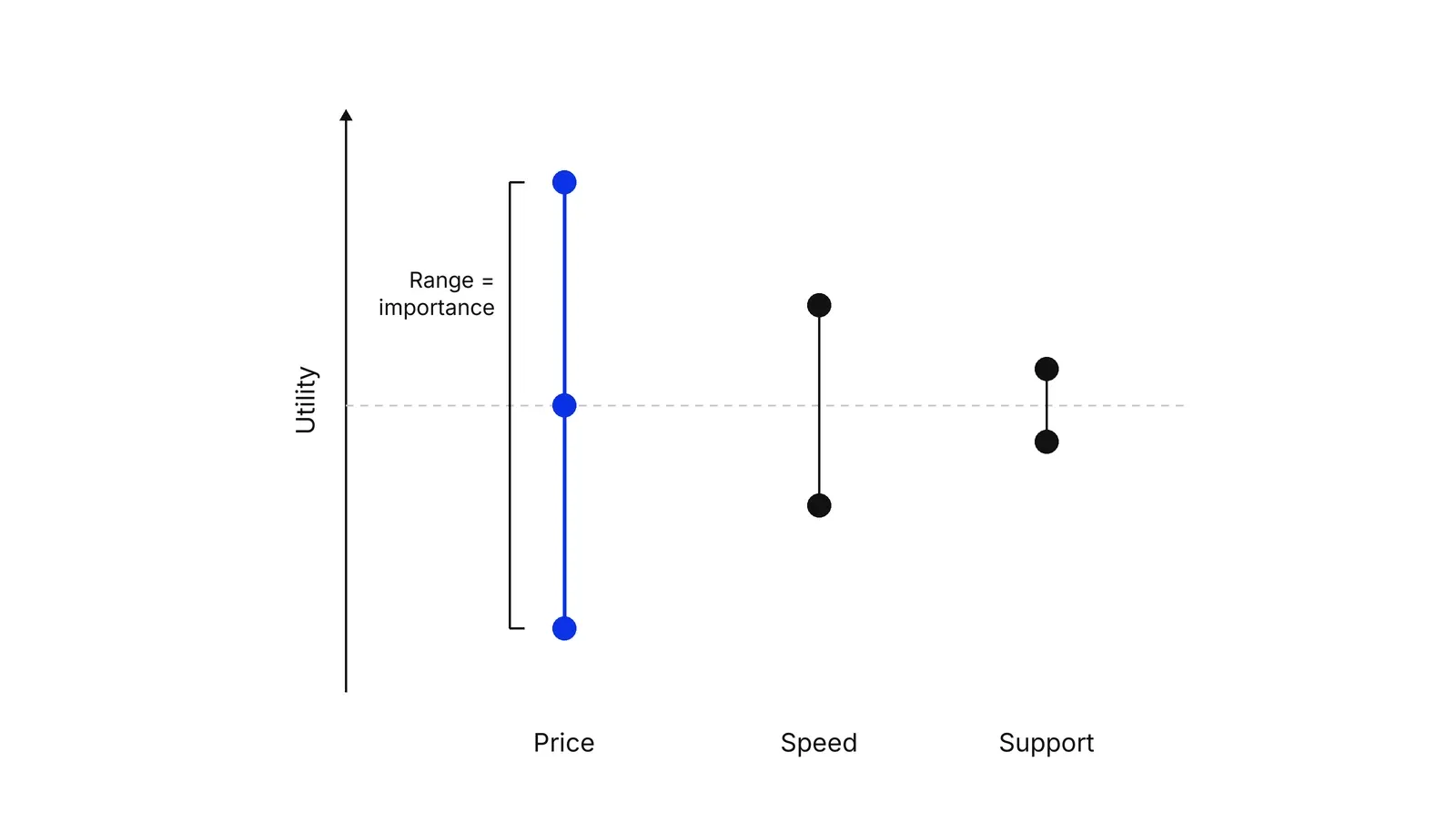
Importance is the range of an attribute’s part-worths divided by the sum of all ranges. Take an illustrative payments study with three attributes. Fee spans 1.8 utility points between $0 and $30, payout speed 0.9 and support 0.3. The total is 3.0, so fee carries three fifths of the importance, speed three tenths and support one tenth.

Importance depends on the levels you chose. Test fees from $0 to $100 and fee will look more important than in a study that tests $10 to $20. Report it with the ranges attached.

Willingness to pay and market simulation

Part-worths let you put a price on a feature. In the payments example, $30 of fee costs 1.8 points, so one dollar is worth 0.06 points. Same-day payout adds 0.9 points over next-day payout, which divides out to about $15 a month.

Treat that figure as an upper bound. Allenby, Brazell, Howell and Rossi (2014) argue that a feature’s economic value is the change in equilibrium profit with and without it, which depends on what competitors offer and what things cost. Their digital camera study found that this measure gives very different answers from the usual willingness-to-pay arithmetic.

A choice simulator is the safer tool. Enter your planned offers and rivals’ current ones, and the model predicts each offer’s share of preference. In the example, a $15 same-day plan with email support and a free next-day rival score the same total utility, so each takes 50%. Add phone support to the paid plan and its share rises to about 57%. Green and Srinivasan (1990) treat simulators as a standard part of the method.

Where results go wrong

Answers are hypothetical, and people are more generous with imaginary money. Ding, Grewal and Liechty (2005) ran conjoint in a restaurant, with participants eating the dinner they chose, and found these incentive-aligned studies predicted later purchases better than hypothetical ones. Where real stakes are impossible, calibrate the simulator against known market shares before trusting it.

Healthcare researchers have formal standards for this. The ISPOR task force published a checklist for conjoint studies in health in 2011 and design guidance in 2013. Political scientists use fully randomized conjoint to estimate the causal effect of each attribute on choices between candidates. In 2012 the Apple v. Samsung patent trial used conjoint surveys run by MIT’s John Hauser to estimate demand for disputed features, according to Sawtooth Software.

Conjoint, MaxDiff and direct price questions

Method	What respondents do	What you get	Best for
Conjoint analysis	Choose between complete profiles	Part-worths, importance, share simulation, price trade-offs	Designing and pricing an offer
MaxDiff	Pick best and worst from 4 or 5 single items	A ranked list of items on one scale	Ranking many features or messages
Van Westendorp	Answer four questions about price	An acceptable price range	Early price range for one product

MaxDiff is the quicker choice when the question is which of 20 features to build first, since respondents only pick the best and worst item from short lists. Conjoint earns its cost when features interact with price. Pushers’ Growth Lab uses it after jobs-to-be-done interviews have named the attributes worth testing.

How to apply Conjoint analysis, step by step

1. Write down the decision. Name the choice the study must settle, such as which of three plans to launch or whether same-day payout justifies a higher fee. A study without a decision produces a pretty chart and no action. Result: one sentence stating the decision and who will make it.
2. Pick attributes and levels from interviews. Run interviews or review support tickets to find the five to eight attributes buyers mention when they compare options. Give each two to five levels that are realistic and that your team could build or charge. Result: an attribute table with levels written in the buyer's words.
3. Build the experimental design. Use conjoint software to generate a balanced design in which every level appears about equally often. Plan enough tasks and respondents that each level is seen at least 500 times across the sample, as Sawtooth Software recommends. Result: a set of choice tasks, each with a few profiles and a None option.
4. Test the survey, then field it. Run the survey with ten people from the target market and watch for tasks they cannot understand or profiles that look absurd. Fix them, then field to at least 300 respondents, with 200 per subgroup you plan to report. Result: clean choice data from the right people.
5. Estimate part-worths and importance. Fit a hierarchical Bayes or multinomial logit model to get a part-worth for every level, then compute each attribute's importance from the range of its part-worths. Check that price part-worths fall as price rises. Result: a table of part-worths and an importance ranking you can explain to the team.
6. Simulate the market and decide. Load the part-worths into a choice simulator, add your offer and the competitors' current offers, and test the options from step one. Compare predicted share and revenue, then make the call. Result: a recommended offer and price, with the simulated share behind it.

Examples

Courtyard by Marriott

In the 1980s Marriott used conjoint analysis to design a new hotel chain. Jerry Wind, Paul Green and colleagues reported in Interfaces in 1989 that the study set the target segments, the service positioning and the room layout. According to John Hauser's 2010 tribute to Green, it covered some 50 features with 160 levels, shown with pictures, three-dimensional models and real rooms where furnishings were varied. Marriott test-marketed the Courtyard concept, then launched it nationally.

Orthodontic clinics in Scotland

Mandy Ryan and Shelley Farrar described a conjoint study in the BMJ in 2000 that asked orthodontic patients in Grampian to trade waiting time (4, 8, 12 or 16 months) against being seen at a local clinic or at the hospital. Respondents preferred local care and would accept about 1.3 extra months of waiting for a local first appointment and about 1.5 months for local follow-up visits. The study had no price attribute, so it priced convenience in months of waiting.

A payments account for online shops

Illustrative, no real company implied. A payments provider tests three attributes: monthly fee ($0, $15 or $30), payout speed (next day or same day) and support (email or phone). The model gives the fee a part-worth range of 1.8 utility points over $30, so one dollar is worth 0.06 points. Same-day payout is worth 0.9 points over next day, which works out to about $15 a month. Phone support adds 0.3 points, about $5. The simulator then shows that adding phone support to a $15 same-day plan moves its share against a free next-day rival from 50% to about 57%.

When to use it

Use it when a team must choose between concrete offer designs or price points before launch, when features interact with price and stakeholders disagree about which matters more, or when you need to estimate how a competitor's move would shift share. It works best for products that buyers already understand, with attributes that can be described clearly in a survey.

When not to use it

Skip it for products so new that buyers cannot judge the attributes, for decisions driven by one attribute alone, and when you have fewer than about 200 reachable respondents. It also cannot tell you which attributes to test; that comes from interviews first. For ranking a long list of features or messages without building whole products, MaxDiff is quicker.

Common mistakes

• Testing attributes the team cares about instead of the ones buyers weigh, because nobody ran interviews before writing the design.
• Using price levels so wide that the cheapest option wins every task, which leaves the model nothing to learn about the other attributes.
• Reading part-worth ratios as the price a market will pay, when competitor offers and costs decide what a feature is worth in practice.
• Packing ten or more attributes into each profile, so respondents start choosing on one or two and ignoring the rest.
• Reporting importance scores as if they were fixed traits of buyers, when they depend on the level ranges chosen for the study.

FAQ

What is conjoint analysis in simple terms?

It is a survey game where people choose between complete products, each built from a mix of features and a price. Because the mixes are varied on purpose, a model can work out how much each feature and price level pushes the choice. The output is a score for every level, which teams use to design and price offers.

What is the difference between conjoint analysis and MaxDiff?

Conjoint shows complete products with several attributes and asks for a choice, so it measures trade-offs and price. MaxDiff shows a short list of single items, usually four or five, and asks for the best and worst. MaxDiff ranks many features or messages quickly but cannot simulate share or price.

How many respondents does a conjoint study need?

Sawtooth Software's rule of thumb is about 300 respondents per study and at least 200 per subgroup you report separately. A second check is that each attribute level should appear at least 500 times across all respondents, with 1,000 a safer target. More attributes and levels raise the number.

How do you calculate willingness to pay from conjoint analysis?

The common shortcut divides a feature's part-worth by the utility of one currency unit taken from the price attribute. Allenby, Brazell, Howell and Rossi showed in 2014 that this can overstate value, because the real worth of a feature depends on competitors' offers and costs. A market simulator gives a more defensible answer.

Why is it called conjoint analysis?

The name comes from conjoint measurement, a branch of mathematical psychology set out by Luce and Tukey in 1964. Conjoint means joined together. A footnote in Sawtooth Software's reissue of Joel Huber's history calls the popular explanation, consider jointly, a misreading. Paul Green named the marketing method in the 1960s.

Sources

1. R. Duncan Luce, John W. Tukey, Simultaneous conjoint measurement: A new type of fundamental measurement, Journal of Mathematical Psychology 1(1), 1964
2. Paul E. Green, Vithala R. Rao, Conjoint Measurement for Quantifying Judgmental Data, Journal of Marketing Research 8(3), 1971
3. Paul E. Green, V. Srinivasan, Conjoint Analysis in Consumer Research: Issues and Outlook, Journal of Consumer Research 5(2), 1978
4. Jordan J. Louviere, George Woodworth, Design and Analysis of Simulated Consumer Choice or Allocation Experiments, Journal of Marketing Research 20(4), 1983
5. Dick R. Wittink, Philippe Cattin, Commercial Use of Conjoint Analysis: An Update, Journal of Marketing 53(3), 1989
6. Jerry Wind, Paul E. Green, Douglas Shifflet, Marsha Scarbrough, Courtyard by Marriott: Designing a Hotel Facility with Consumer-Based Marketing Models, Interfaces 19(1), 1989
7. Paul E. Green, V. Srinivasan, Conjoint Analysis in Marketing: New Developments with Implications for Research and Practice, Journal of Marketing 54(4), 1990
8. Peter J. Lenk, Wayne S. DeSarbo, Paul E. Green, Martin R. Young, Hierarchical Bayes Conjoint Analysis, Marketing Science 15(2), 1996
9. Jordan J. Louviere, David A. Hensher, Joffre D. Swait, Stated Choice Methods: Analysis and Applications, Cambridge University Press, 2000
10. Mandy Ryan, Shelley Farrar, Using conjoint analysis to elicit preferences for health care, BMJ 320, 2000
11. Paul E. Green, Abba M. Krieger, Yoram Wind, Thirty Years of Conjoint Analysis: Reflections and Prospects, Interfaces 31(3 suppl.), 2001
12. Joel Huber, Conjoint Analysis: How We Got Here and Where We Are (An Update), Sawtooth Software Research Paper Series, 2005
13. Min Ding, Rajdeep Grewal, John Liechty, Incentive-Aligned Conjoint Analysis, Journal of Marketing Research 42(1), 2005
14. John R. Hauser, Paul E. Green: An Applications' Guru, MIT Sloan School of Management, 2010
15. John F. P. Bridges et al., Conjoint Analysis Applications in Health: a Checklist, ISPOR Task Force report, Value in Health 14(4), 2011
16. F. Reed Johnson et al., Constructing Experimental Designs for Discrete-Choice Experiments, ISPOR Task Force report, Value in Health 16(1), 2013
17. Jens Hainmueller, Daniel J. Hopkins, Teppei Yamamoto, Causal Inference in Conjoint Analysis, Political Analysis 22(1), 2014
18. Greg M. Allenby, Jeff D. Brazell, John R. Howell, Peter E. Rossi, Economic valuation of product features, Quantitative Marketing and Economics 12(4), 2014
19. Vithala R. Rao, Applied Conjoint Analysis, Springer, 2014
20. Jordan J. Louviere, Terry N. Flynn, A. A. J. Marley, Best-Worst Scaling: Theory, Methods and Applications, Cambridge University Press, 2015
21. Wharton Magazine, The father of conjoint analysis: Paul Green
22. University of Pennsylvania Almanac, Obituary of Paul E. Green, October 2012
23. Sawtooth Software, Choice-Based Conjoint (CBC)
24. Sawtooth Software, Sample size rules of thumb for conjoint analysis
25. Sawtooth Software, Results of the Sawtooth Software user survey, 2019
26. Sawtooth Software, 5 examples of conjoint analysis studies in the real world
27. Sawtooth Software, MaxDiff

Last updated Oct 9, 2026